January 2021 Vol. 76 No. 1

Features

CIGMAT Report: Transferring Technology from Control Studies to Actual Applications

Real-time monitoring during construction, entire service life, and detecting and quantifying corrosion for maintenance are some of the major focus areas of the CIGMAT research related to oil, gas, water and wastewater infrastructures, bridges, foundations and pipelines. These goals are achieved by developing new, highly sensing smart materials for construction, maintenance, repairs and detection of gas, oil and water leaks, which recently received a U.S. Patent (Number 10,481,143). Other studies on detecting and quantifying corrosion also recently received a U.S. Patent (Number 10,690,586). 

Current projects at the CIGMAT Research Center are developing real-time monitoring systems for laboratory research and field applications, both onshore and offshore. These include monitoring field performances (smart cemented well, bridges support on deep foundations); developing and characterizing smart cements, smart grouts and smart drilling muds for oil well and water well construction and cementing; ultra-deepwater pipe-soil interaction; joint leak testing of storm water pipes; detection and quantification of corrosion; and application of nanotechnology. 

In recent years, CIGMAT researchers have developed unique testing facilities, such as high pressure and high temperature (HPHT) testing of materials for oil and gas infrastructure applications, and test protocols approved by the U.S. Environmental Protection Agency to test grouts and coatings for infrastructure rehabilitations. The Life Cycle Cost model for wastewater systems, available on the CIGMAT website (http://cigmat.cive.uh.edu.) is being used by cities, counties and the public. 

Over the past two decades, more than five dozen commercial products, including rapid repair materials, coatings, grouts, liners, cementitious and polymer composites and pipes, have been researched and tested for numerous applications. Also, microbial fuel cell technology is being further developed to treat both oily waste and recycle highly salty fracturing fluids. 

Researchers analytically and numerically model observed trends to better understand the influence of various testing and environmental parameters. The Vipulanandan rheological and Vipulanandan failure models, for example, are being verified with CIGMAT test results and data. Every effort is being made by the CIGMAT researchers to transfer technology from control studies to actual applications. 

Ongoing research at CIGMAT is funded by federal, state and local agencies, and industries. This includes projects funded by the U.S. Department of Energy and National Science Foundation to broaden applications of smart cement and smart drilling mud for real-time monitoring of oil well installation and performance over the entire service life, as well civil infrastructure applications. 

Smart cement is also being used as the binder in developing and characterizing concrete. Several systems are being used to monitor performance of the cement sheath that is embedded between the casing and geological formations. 

During CIGMAT’s annual Conference and Exhibition, “Infrastructures, Energy, Geotechnical, Flooding and Sustainability Issues Related to Houston and Other Major Cities,” in early March, speakers from major cities, transportation authorities and energy industries around the country present and discuss projects and problems related to construction, maintenance and rehabilitation issues. 

The well-attended conference also covers technical issues related to maintenance and rehabilitation of water and wastewater systems, nondestructive testing methods, oil wells and pipelines, hydraulic fracturing, and development of smart materials for various applications. In addition, numerous geotechnical topics regarding expansive clays, rapid construction of deep foundations and ground faulting are discussed. The Proceedings of the past 20 years of conferences are posted on the CIGMAT website: http://cigmat.cive.uh.edu. 

STEEL CORROSION DETECTION AND QUANTIFICATION REAL-TIME USING A NEW NONDESTRUCTIVE TESTING METHOD (U.S. PATENT NUMBER 10,690, 586) 

A major challenge facing the aging infrastructure is material loss and deterioration due to corrosion. Many studies indicate that in the US alone, costs due to corrosion loss is more than $276 billion annually. In the oil and gas industry, annual costs in the U.S. are over $27 billion and globally are $60 billion. 

Corrosion is the major cause of deterioration of steel structures and components. For example, corrosion of load-bearing steel piles that are used as foundations for various types of structures, may result in reduced capacity in the axial and lateral directions. Hence, understanding the rate of steel corrosion is essential to designing the steel-based facilities to avoid excessive deflection and failure. 

Defined as the deterioration of a material because of the continuous bio-chemo-stress-thermo reactions with the environment, corrosion occurs in practically all environments – to some degree. For steel, moisture, water, acids, gases, soil, biological activities, thermal cycling and stress variations can cause the degradation of material properties. In the petroleum industry salts, acids, and water are more corrosive than the oil. 

Corrosion occurs in unprotected steel structures in any location and varies in intensity depending on local variables. Accelerated Low Water Corrosion (ALWC) is defined as the localized and aggressive corrosion phenomenon that typically occurs at or below low-water level and is associated with microbially induced corrosion. ALWC corrosion rates are typically 0.5 mm/side/year averaged over time to the point of complete perforation of steel plate. This corrosion process can be significantly affected by bacterial activity and fluctuating water table, in addition to the condition of the soil. 

To prevent the deterioration mechanisms that affect steel, it is essential to identify and understand what causes the damage. It is widely recognized that the corrosion of carbon steel in soil, water and soil-water interface proceeds according to the following simplified anodic reaction and cathodic reactions in the presence of oxygen and water. 

Anode: Fe t Fe2+ + 2e– (1) 

Cathode: O2 + 2H2O + 4e– t 4OH– (2) 

Therefore, the overall chemical reaction is Fe2+ + 4OH– + O2 t Fe2O3 (Rust) + H2O. 

When the Fe atoms that leave the surface at the anode as Fe2+ move into the environment, they form small pitting holes at the anode. But when the released Fe2+ ions remain on the cathodic surface, it leads to large depositions of rust. These deposits form a hard mass that doesn’t have the mechanical strength and is very brittle. 

The potential of the corroding electrode (anode) with respect to a reference electrode is called corrosion potential. The current established due to the corrosion reaction is called the corrosion current and the degree of corrosion directly relates to the rate of corrosion occurring at the surface. 

Over the past 20 years, there has been growing awareness of an accelerated form of corrosion concentrated around the low-water mark of maritime structures. This ALWC is a rapid pitting form of microbial-induced corrosion (MIC) that occurs more rapidly than others previously identified. 

The most common variety of ALWC occurs as a horizontal band around low water, but it can also be found in patches, and extends down to bed level. The appearance and characteristics of ALWC are generally recognizable as lightly adherent orange and black corrosion products over otherwise clean steel. 

Corrosion changes the material properties of the steel, decreasing its strength and changing its microstructure. Hence, it is important to be able to detect and evaluate the extent of corrosion of the steel surface. Evaluation methods employed are visual inspection, weight loss measurements, material composition variation, ultrasonic method, and studies of the structure of the deposition material using XRD measurements. 

Objectives, materials & methods 

The overall objective was to develop and demonstrate the potential of the new nondestructive corrosion detection and quantification method using steel specimens. Specifically, objectives were to: 

• Identify the equivalent electrical circuits for the surface and bulk corrosion of steel and represent them in terms of electrical properties using the impedance frequency relationship.
• Investigate the corrosion of steel specimens with time placed in 10% salt solution and quantify the surface and bulk corrosions along the length of the steel specimens.
• Compare the weight loss due to corrosion with the changes in the electrical properties used to quantify the corrosion.

The material used was ASTM A1018 Mild steel. For the weight loss study, the samples were 76 mm in length. For the electrical characterization of corrosion, the steel bars were 750 mm (30 inches) long, 30 mm wide and 4.1 mm thick. The chemical composition of the steel is summarized in TABLE 1. 

For the accelerated test, 10% sodium chloride (NaCl) solution was used for corroding the specimens. The steel specimens were placed in this solution in a plastic container for the entire duration (500 days) of testing. 

Theory and Concepts 

In this study, an equivalent circuit to represent the corrosion was required for better characterization, through the analyses of the impedance spectrocopy data. There were many difficulties associated with choosing the most-appropriate equivalent circuit, such as linking the different elements in the circuit and the different regions in the impedance data of the corresponding sample. 

As a result, different possible equivalent circuits were analyzed to find an appropriate equivalent circuit to represent the corroding steel, using the two-probe monitoring. 

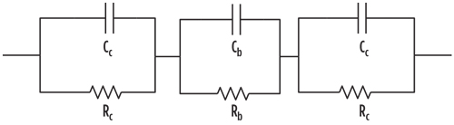
In the equivalent circuit for CASE-1, the contacts were connected in series, and both the contacts and the bulk material were represented using a capacitor and a resistor connected in parallel, as shown in FIGURE 1. 

Rb and Cb are resistance and capacitance of the bulk material, respectively; Rc and Cc are resistance and capacitance of the contacts, respectively. Both contacts are represented with the same resistance (Rc) and capacitance (Cc) as they are identical. Total impedance of the equivalent circuit for CASE-1 (Z1) can be represented as follows: 

 

(3)

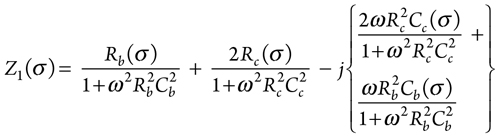
where ω is the angular frequency of the applied alternative current (AC) signal. 

When the frequency of the applied signal was very low, ω t 0, Z1 = Rb + 2Rc, and when it is very high, ω t ∞, Z1 = 0. 

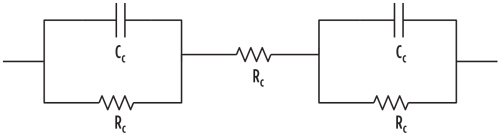
In CASE-2, as a special case of CASE-1, the capacitance of the bulk material (Cb) was assumed to be negligible, as shown in FIGURE 2. 

The total impedance of the equivalent circuit for CASE-2 (Z2) is as follows: 

 

 

(4) 

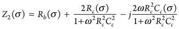
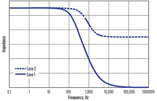
When the frequency of the applied signal was very low, ω t 0, Z2 = Rb + 2Rc, and when it is very high, ω t ∞, Z2 = Rb as shown in FIGURE 3. 

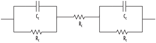
In the case of corrosion measurement, the two contacts will have different properties and will be represented as shown in FIGURE 4. 

CASE-2 equivalent circuit was used to determine the contact electrical resistances (Ri, Rc) and contact capacitances (Ci, Cc) at the surface between the steel bar and the two probes. During the impedance characterization, at least 15 data collected for each test was used to determine the five unknowns in Equation (5): 

 

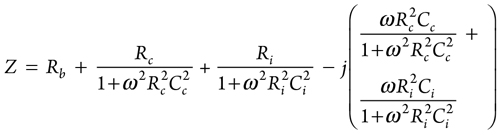
(5) 

The resistance (R) and capacitance (C) for the bulk material between two points of measurements are defined as: 

 

 

 

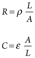
(6) (7) 

where A = cross-sectional area, L = distance between the two probes, ρ = resistivity of the material and ε = absolute permittivity of the material 

The product of Equations (6) and (7) results as 

RC = ρε. (8) 

Since ρ and ε in equations (6) and (7) are material properties, RC at the point of contact is also a material property and is referred as Vipulanandan contact/corrosion index. This parameter will be used in characterizing the surface corrosion at the points of contacts of the measuring probes. 

Measuring the electrical resistivity of the steel specimen was a challenge due to the unknown path of electron flow inside the steel specimen. Hence, resistance was used as a measuring variable to determine the steel’s electrical resistivity. 

Resistance was measured at high frequency (300 kHz) using the two magnetic probes (Contact 1 and 2), as shown in FIGURE 5, and was correlated to the electrical resistivity of the steel specimen using the effective K factor in Equation (6) for a period of one year. 

The effective K factor that determined the electrical resistivity of the steel was obtained from Equation (6) using the initial resistance of the steel measured on day 1 via the LCR meter and theoretical electrical resistivity of the steel is ρ0 = 1.59 E–07 Ωm. Bulk steel electrical resistivity of the corroded specimen was calculated using Equation (6), after getting the bulk resistance from Equation (5). 

Steel specimen electrical resistivity (ρ) and resistance (R) relationship in Equation (6) can be represented with the increments ∆ρ and ∆R as follows: 

 

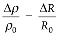
(9) 

ρ = ρ0 + ∆ρ. (10) 

Results and discussion 

Steel samples with a dimension of about 76 mm (length) × 30.54 mm (width) × 4.14 mm (thickness) were used for this experiment. Specimens were placed in 10% sodium chloride solution and tested regularly. At every cycle, weight and dimension of the specimen were noted. 

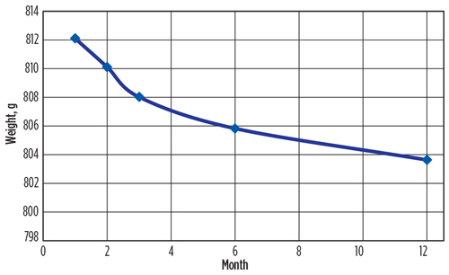
According to ASTM G1-90 standard, the specimens were cleaned, and the weight and the dimensions were measured to estimate the corrosion rate. As shown in the FIGURE 6, the average weight of the corroding steel specimens reduced from 812.1 g to 803.6 g in one year of corrosion, or 1.05%. The corrosion rate varied with time and the average was about 3.8 × 10–7 mm/year. 

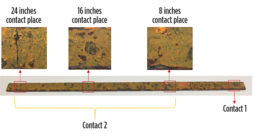
The impedance-frequency measurements were performed on a weekly basis for 500 days. The tests were done at three location along the steel, indicated as Contact 2 in FIGURE 7; Contact 1 was the same for all three cases. The frequency range was 20 Hz to 300 kHz. 

The observed shape of the impedance-frequency curve represented CASE-2; the bulk material steel (inner layer) was represented as resistance and the contacts on the surface of the steel (outer layer) as a parallel combination of resistance and capacitance. The total impedance of the electrochemical system increased continuously with time. The corroded steel bar after 1 year in the salt solution is shown in FIGURE 7. 

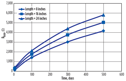
The observed shape of the impedance curve indicated the conductive steel was becoming more resistive, as the shape of the curve represented CASE-2 in FIGURE 3. The steel specimen’s resistance also increased with time, as shown in FIGURE 8: 

• For 8-inch distance, bulk resistance increased from 0.111 Ω to 4613 Ω in 500 days of corrosion, which showed a tremendous change of 41,558 times.
• For 16- inch distance, bulk resistance increased from 0.124 Ω to 5042 Ω, showing a change of 40,661 times.
• For 24-inch distance, bulk resistance increased from 0.131 Ω to 5810 Ω, showing a change of 44,351 times.

All these changes indicated that the inner layer of steel was also corroding, which would not be reported and quantified in other corrosion experiments. 

This increasing trend of the curve, as shown in FIGURE 8, indicated the rate of corrosion was slightly decreasing, but the corrosion process was continuing. As the rust is an oxide compound, an increase in corrosion or rust formation causes the resistance and resistivity of the material to increase. 

At lower frequencies, the impedance values were high because of the enormous corroding contact resistance (resistance due to rust layer); at a higher frequency, the curve was dominated by the bulk resistance. The phase angle of the impedance increased with time, which clearly indicates its capacitive behavior. Change in the phase angle of the contacts also indicated the corrosion was taking place. 

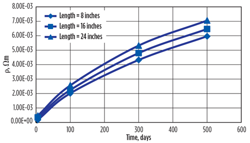
The resistivity of the corroding steel specimen measured using nondestructive corrosion sensing technique is shown in FIGURE 9 for the 500-day testing period. The resistivity of the material was calculated using Equations (9) and (10) and indicates a high corrosion level. 

Resistivity increases from 1.59 × 10–7 Ωm to 5.96 × 10–3 Ωm for the 8-inch length, from 1.59 × 10–7 Ωm to 6.47 × 10–3 Ωm for the 16-inch length, and from 1.59 × 10–7 Ωm to 7.05 × 10–3 Ωm for the 24-inch length, during the 500-day testing period. These values also indicate that the metal is turning from conductive to the insulative material. As the corrosive ions are getting depleted, we could see the drop in corrosion rate as time increases, thus, proving the accuracy of the corrosion measurement. 

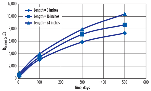
The variation of resistance for the three Contact-2 locations (FIGURE 7) are shown in FIGURE 10 for the testing time period of 500 days. It could be observed that the contact resistances were increasing with time and had progressively higher corrosion product. Visually, FIGURE 7 shows a crack with a very loose surface layer at the 24-inch contact, indicating more corrosion. The 16-inch contact has a corrosion pit and the 8-inch has a smooth, rust layer. 

This makes the nondestructive electrical corrosion sensing method more reliable with its accurate results. Resistance value of Contact-2 increased from 0.07 Ω to 7322 Ω during the 500-day testing period at the 8-inch location, from 0.07 Ω to 8658 Ω at the 16-inch location, and from 0.07 Ω to 10388 Ω at the 24-inch location, indicating a high corrosion level. 

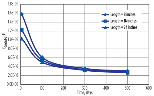
The capacitance at Contact-2 on the steel surface (CC2), shown in FIGURE 14, decreases with the increasing corrosion period. Similar to Contact-1, the curvature of the plot increases with the increase in the corrosion period, and gradually becomes flat, indicating very low contact capacitance, or increasing resistance to corrosion, or a decreasing corrosion rate. 

The higher change was observed with Contact-2 capacitance, compared to the Contact-1 surface, where capacitance value decreased from 1.58 E–09 F to 3.06 E–10 F at the 8-inch measurement, from 1.22 E–09 F to 2.82 E–10 F at 16 inches, and from 1.03 E–09 F to 2.67 E–10 F at 24 inches. 

The higher RcCc value of Contact-1 (FIGURE 7) indicates the steel specimen is corroding, but Contact-2 corrosion is even higher. This difference indicates the accuracy of the method to separate the contacts’ material properties and denote the characteristics. RC1CC1 value of the steel specimen increases from 1.51 E–06 ΩF to 1.82 E–05 ΩF showing a great deal of corrosion. 

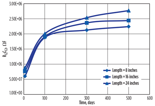
The corrosion index parameter RC2CC2 value at the 8-inch location increased from 5.97 E–07 ΩF to 2.24 E–06 ΩF (275% increase) during the 500-day testing period and the 16-inch location increased from 7.57 E–07 ΩF to 2.44 E–06 ΩF (222% increase). At the 24-inch location, the corrosion index parameter increased from 8.72E–07 ΩF to 2.77E–06 ΩF – the highest corrosion index. Based on the visual results (FIGURE 7), corrosion was also higher at 24 inches, compared to the other two locations. 

In addition, the RC2CC2 at the 16-inch location was higher than the 8-inch location. So all the contact indices, representing the Vipulanandan corrosion index, could be easily tied to the visual corrosion observation in FIGURE 7. 

This proves the sensing nature of this method at different locations. The new electrical method can quantify the surface corrosion very well. 

Conclusions 

Based on the steel corrosion monitored for 500 days with the electrical method, the following can be deduced: 

• The weight change in 10% salt solution in one year was 1.05%.
• Resistivity of the steel specimen subjected to marine corrosion for a period of 500 days in 3.55 salt solution, changed more than 40,000 times (4,000,000%) – highly sensitive compared to weight change.
• A material property that characterizes the surface corrosion was determined to be the product of resistance and capacitance, Vipulanandan corrosion index.
• The material property, contact index RcCc of the three Contact-2 locations increased due to corrosion of the steel, changing by over 200%.
• All the impedance characterization results were comparable to the visual corrosion method, proving the reliability of the nondestructive electrical corrosion sensing method.

SMART CEMENT WITH 1% NanoSiO2 

Past studies have shown that adding nanoparticles have a strong influence on the mechanical and electrical properties of the cementitious materials, including all types of cement and cement concrete. Because the nanoparticles have a relatively large surface area, there will be higher chemical reactivity and the dispersed nanoparticles will fill the voids between the hydrating cement particles, resulting in denser cement. 

Also, the well-dispersed nanoparticles act as crystallization centers, based on the chemical composition, accelerating the cement hydration, producing additional quantity of calcium silicate hydrate (C−S−H) and promoting crystallization of small-sized calcium hydroxide (Ca (OH)2) crystals. Hence, it is important to investigate the effects of adding nanoparticles on the behavior of the highly sensing chemo-thermo-piezoresistive smart cement (U.S. Patent Number 10,481,143). 

One of the most useful nanomaterials is nanosilica. Based on the improved compressive strength, it is clear that NanoSiO2 behaves not only as a filler to improve the cement microstructure, but also to promote the pozzolanic reactions. Therefore, it is of interest to add NanoSiO2 particles to the cement mixtures to enhance performance. Also adding NanoSiO2 decreased the amount of lubricating water available in the mixture. 

Nano-scaled silica particles have a filler effect by filling up the voids between the cement grains. With the right composition, the higher packing density results in a lower water demand of the mixture and contributes to strength enhancement due to the reduced capillary porosity. 

The overall objective of this study was to investigate the effect of up to 1% of NanoSiO2 on the chemo-thermo-smart cement behavior. Smart cement samples were prepared with class H cement and w/c ratio of 0.38. 

Silicon dioxide nano powder (NanoSiO2) with grain size of 12 nm and specific surface area of 175 to 225 m2/g (from supplier datasheet) was selected for this study. 

Results and discussion 

The average density of the smart cement with less than 0.1% carbon fiber was 1.975 g/cc (16.47 ppg). The initial electrical resistivity (ρo) of the smart cement mix with w/c ratio of 0.38 was 1.06 Ωm. 

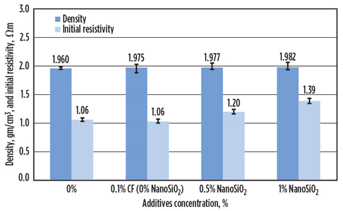
The average density of the smart cement with 0.5% NanoSiO2 was 1.977 g/cc (16.49 ppg), a 0.1% increase. The initial electrical resistivity (ρo) of this smart cement was 1.20 Ωm, a 13% increase, as shown in FIGURE 13. The resistivity was more sensitive to the addition of NanoSiO2 than the density. 

The average density of the smart cement with 1% NanoSiO2 was 1.982 g/cc (16.53 ppg), about a 0.4% increase. The initial electrical resistivity (ρo) of this smart cement was 1.39 Ωm, a 31% increase, as shown in FIGURE 13. The resistivity was more sensitive to the 1% NanoSiO2 addition than the density. 

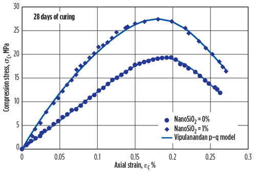
The compressive stress-strain relationships for the cement with and without NanoSiO2 and cured for 28 days are shown in FIGURE 14. Based on the experimental results, the Vipulanandan p-q stress-strain model was used to predict the relationship as follows: 

 

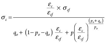
(11) 

 

where: σc is compressive stress and εc compressive strain; σcf and εcf are the compressive strength and corresponding strain as summarized in TABLE 2. The model parameters po, and qo are also summarized in TABLE 2. Model parameters po and qo increased with curing time based on the NanoSiO2 content. 

The compressive strength (σcf) of the smart cement after 28 days of curing was 19.3 MPa (2,800 psi), as shown in FIGURE 14. The failure strain was 0.22% and the initial modulus was 12,500 MPa (1.8 × 106 psi), as summarized in TABLE 2. The model parameters qo and po were 0.70 and 0.160 respectively. The parameter qo represents the nonlinearity up to peak stress, and the smart cement had the highest linearity, highest value of parameter qo as shown in FIGURE 14. The coefficient of determination (R2) was 0.99 and the root-mean-square error (RMSE) was 0.110 MPa as summarized in TABLE 2. 

The compressive strength (σcf) of the smart cement with 1% NanoSiO2 after 28 days of curing was 27.5 MPa (4,000 psi), 42.5% higher than the smart cement without NanoSiO2 as shown in FIGURE 14. The failure strain was 0.19% and the initial modulus was 25,400 MPa (3.7 × 106 psi) as summarized in TABLE 2. Addition of 1% NanoSiO2 to the smart cement reduced the failure strain and increased the modulus compared to the smart cement without NanoSiO2. 

The model parameters qo and po were 0.57 and 0.100, respectively. The parameter qo represents the nonlinearity up to peak stress and was lower than the smart cement without NanoSiO2 as shown in FIGURE 14. The coefficient of determination (R2) was 0.99 and the root-mean-square error (RMSE) was 0.150 MPa as summarized in TABLE 2. 

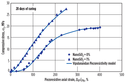
Based on experimental results, Vipulanandan p-q piezoresistivity model was used to predict the change in electrical resistivity of cement with applied compressive stress for 28 days of curing. The model is defined as follows: 

 

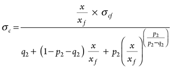
(12) 

 

where σc is the stress (MPa); σcf is the compressive strength at failure (MPa); x = (∆ρ/ρo) × 100 : Percentage of piezoresistive axial strain to the stress; xf = (∆ρ/ρo)f × 100 : Percentage of piezoresistive axial strain at failure; ∆ρ: change in electrical resistivity; ρo : initial electrical resistivity (σ = 0 MPa) and p2 and q2 are the piezoresistive model parameters. 

The piezoresisitive axial strain of the smart cement at failure (∆ρ/ρo)f after 28 days of curing was 400%, as summarized in TABLE 3 and shown in FIGURE 15. The compressive axial failure strain was 0.22%, so the axial strain increased by 1,818 timpiezoresistivees (181,800%), making the smart cement highly sensing. The model parameters q2 and p2 were 0.05 and 0.03, respectively. The coefficient of determination (R2) was 0.99 and the root-mean-square error (RMSE) was 0.022 MPa as summarized in TABLE 3. 

The piezoresisitive axial strain of the smart cement with 1% NanoSiO2 at failure (∆ρ/ρo)f after 28 days of curing was 250%, as summarized in TABLE 3 and shown in FIGURE 15. Addition of 1% NanoSiO2 reduced the piezoresistive axial strain at failure of the smart cement by 37.5%. 

The compressive axial failure strain was 0.19%, so the piezoresistive axial strain was increased by 1,316 times (131,600%), making the smart cement highly sensing. The model parameters q2 and p2 were 0.35 and 0.14, respectively. The coefficient of determination (R2) was 0.99 and the root-mean-square error (RMSE) was 0.016 MPa, as summarized in TABLE 3. 

Conclusions 

Based on the experimental and analytical study on the smart cement modified with silica nanoparticles (NanoSiO2) up to  
1%, the following conclusions are advanced: 

• Addition of 1% NanoSiO2 increased the density (by 0.4%) and the initial resistivity (by 31%) of the smart cement.
• Addition of 1% NanoSiO2 increased the compressive strength of the smart cement by 42% after 28 days of curing and the modulus of elasticity of the smart cement increased. The Vipulanandan p-q stress-strain model predicted the behavior very well.
• Addition of 1% NanoSiO2 reduced the piezoresistive axial strain at failure of the smart cement. The Vipulanandan p-q piezoresisitive model predicted the behavior very well.

 

The 25th CIGMAT-2021 Conference and Exhibition will be held on March 5, 2021, as an online event. Check the CIGMAT website for details and updates: cigmat.cive.uh.edu 

 

From Archive